Rasterizer

Overview

Give a high-level overview of what you implemented in this project. Think about what you’ve built as a whole. Share your thoughts on what interesting things you’ve learned from completing the project.

With this project, I learned about the rasterization process in the graphics pipeline. We were expected to implement the rasterization of triangles, supersampling feature to reduce the jaggies, and various ways to set the color of each pixels in the rasterized triangle.

I’ve found the direct application of math and geometry fascinating. The project was especially rewarding as the feedback on whether the implementation is correct is immediate and visual.

I attach the following as an interesting memeory while progressing through the project.

Task 1

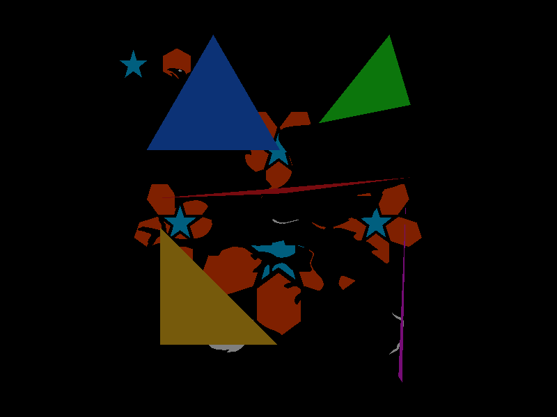
Walk through how you rasterize triangles in your own words. Explain how your algorithm is no worse than one that checks each sample within the bounding box of the triangle. Show a png screenshot of basic/test4.svg with the default viewing parameters and with the pixel inspector centered on an interesting part of the scene.

When sampling the pixels, I check the bounding box of a triangle rather than the whole screen. I made a bit of optimization in the extra credit section, reducing the times the pixel sampling routine is called.

The part that is zoomed in is interesting because we can see the jaggies and an isolated point in what seemingly should be a solid red triangle. As we will find out, in the task 2 we will implement a supersampling method to reduce these artifacts.

Each pixels in the bounding box is checked for its inclusion in the triangle being evaluated. To check the wether the pixel that’s sampled is within the triangle, a three line test is performed as described in the lecture. When all three tests confirm a point is within the triangle, fill_pixel function is called with the color we want to fill the pixel with, which writes the information to the frame buffer.

Extra credit

Extra credit: Explain any special optimizations you did beyond simple bounding box triangle rasterization, with a timing comparison table (we suggest using the c++ clock() function around the svg.draw() command in DrawRend::redraw() to compare millisecond timings with your various optimizations off and on).

The code for extra credit portion of the Task 1 can be found under the task1_extracredit branch. The performance data can be found in this document under Attachments > Task 1 Extra Credit Data.

I initially implemented the bounding box checking method to ensure we are not sampling the whole screen for every triangle. From there, I wanted to use the fact that within the bounding box, we know there are strides of continuous hits that are bound to happen due to the geometry of triangle (it’s convex).

So I made a stride parameter and adapted the point evaluation loop in the code base to adjust accordingly. When the mechanism detects the strides, instead of checking each sample points, it processes the stride without sample all of the elements within the stride.

I’ve included the results of the strides of 4 and 8. Interestingly, when stride was set to 8 the performance worsened, and that likely is due to lowered stride hit rates thus increased overhead with small triangles.

Results: With the image rendered with 4 unit stride mechanism, basic/test6.svg saw 7.2% improvement in rendering time, and basic/test3.svg saw 4.32% improvement in rendering time.

Note: there are variations in the execution time on a real machine - the performance metric could be improved to run 1000 times and report an average and a standard deviation of the execution times.

Also Note: the initial implementation of the line evaluation was not so poor! So small percentage improvement is expected!

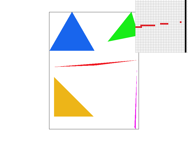
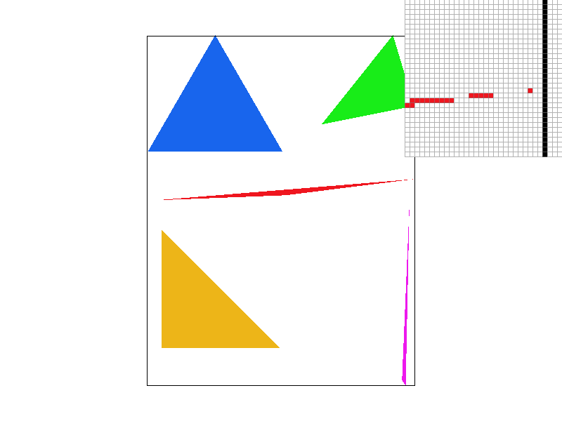
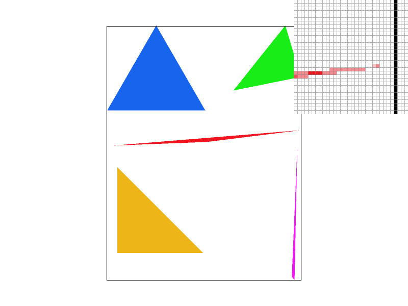
You can see the stride operation in the below right image, obtained by only coloring the long strides. On the left side, we could see the original bounding box evaluation scheme. If the image is too small, right-click and view the images separately in a new window.

Task 2

Walk through your supersampling algorithm and data structures. Why is supersampling useful? What modifications did you make to the rasterization pipeline in the process? Explain how you used supersampling to antialias your triangles.

Supersampling allows for the cases where an edge of the triangle is not quite covering the full surface of a pixel which can lead to ‘jaggies’ on the screen. See below image “Supersampling Rate: 1”.

supersample_buffer vector data structure which holds ‘arrays’ of Color structs is used to hold the Color values before being combined/average and drawn onto the frame buffer. The supersample_buffer needs to be updated every time, the supersampling rate changes by an user input, or when the screen size changes.

The Task 1 code (rasterize_triangle) was updated to evaluate the triangles at sub-pixel level. Instead of calling fill_pixel when the sample needs to be filled, fill_supersample function is called instead. unsigned int sample_rate is used to dynamically adjust the sub-pixel sampling loop.

After the rasterization into the supersample_buffer is done, the resolve_to_framebuffer function is called to resolve supersampled values at a pixel, and draw the pixel onto the screen by writing to the frame buffer.

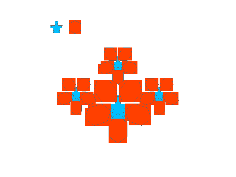
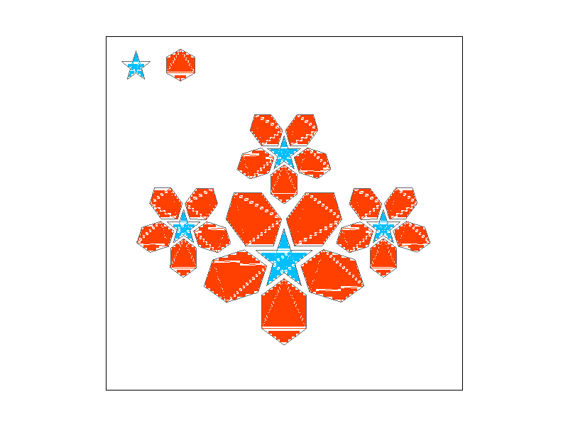
Show png screenshots of basic/test4.svg with the default viewing parameters and sample rates 1, 4, and 16 to compare them side-by-side. Position the pixel inspector over an area that showcases the effect dramatically; for example, a very skinny triangle corner. Explain why these results are observed.

As one can observe below, as the supersampling rate increases, we can see each pixels around the rough jaggied area getting blurred. This is the artifact of samplling at granular level than 1 per pixel and combining (or ‘blend in’) the results to render that single pixel.

Task 3

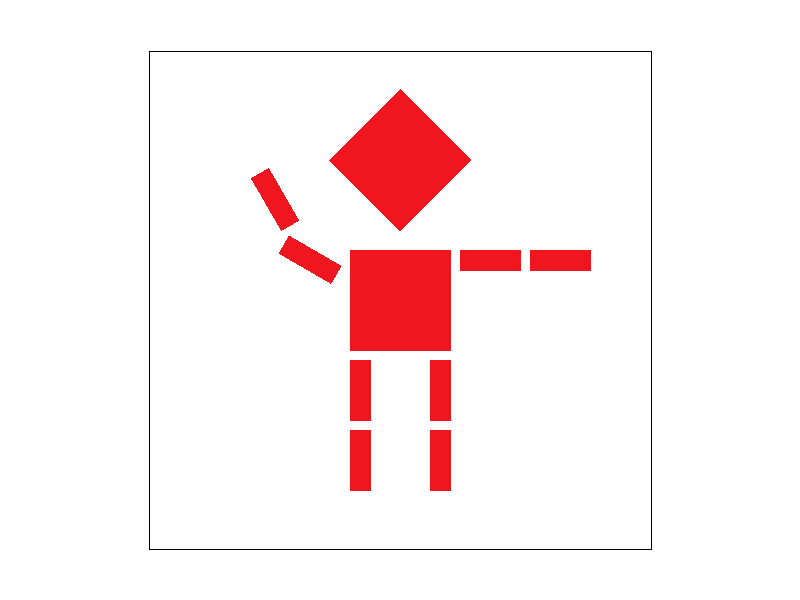
Create an updated version of svg/transforms/robot.svg with cubeman doing something more interesting, like waving or running. Feel free to change his colors or proportions to suit your creativity. Save your svg file as my_robot.svg in your docs/ directory and show a png screenshot of your rendered drawing in your write-up. Explain what you were trying to do with cubeman in words.

A robot is waving hello. He also got a CPU upgrade (bigger head). I initially implemented the robot incorrectly as the trig functions in gcc takes radian, but the transform functions in the codebase uses degrees.

Link to robot waving SVG file: Here

I rotated the arm components so that it looks like robot is waving, and translated and scaled the head to be big!

Task 4

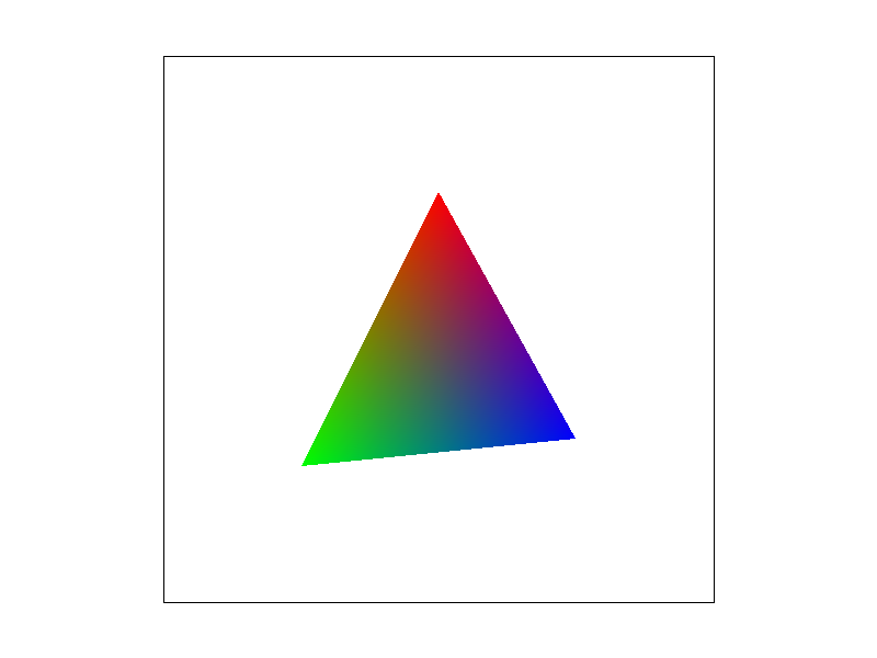
Explain barycentric coordinates in your own words and use an image to aid you in your explanation. One idea is to use a svg file that plots a single triangle with one red, one green, and one blue vertex, which should produce a smoothly blended color triangle.

As one can see below, each triangle’s corners are colored red, green and blue. With barycentric coordinate, we can interpolate the values within (and outside, but we are interested in the inner side*) the triangle. In the example below, the colors on the each corners are interpolated and inner pixels of the triangles are filled appropriately.

*when the barycentric coordinates are all positive

Show a png screenshot of svg/basic/test7.svg with default viewing parameters and sample rate 1. If you make any additional images with color gradients, include them.

Task 5

Explain pixel sampling in your own words and describe how you implemented it to perform texture mapping. Briefly discuss the two different pixel sampling methods, nearest and bilinear.

To pixel sample, for each screen sample with barycentric coordinate, evaluate the texture coordinate and sample the texture. For the nearest method, once you evaluate the texture coordinate, round the value to the nearest pixel in the texture coordinate. For the bilinear method, once you evaluate the texture coordinate, interpolate the colors between four pixels around the sample point as described in the lecture.

We use the zero level of the mipmap (the full texel resolution) to render the images in this task and this could lead to aliasing, but that will be dealt in task 6.

Check out the svg files in the svg/texmap/ directory. Use the pixel inspector to find a good example of where bilinear sampling clearly defeats nearest sampling. Show and compare four png screenshots using nearest sampling at 1 sample per pixel, nearest sampling at 16 samples per pixel, bilinear sampling at 1 sample per pixel, and bilinear sampling at 16 samples per pixel.

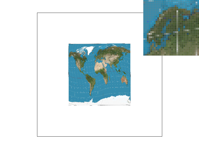
Comment on the relative differences. Discuss when there will be a large difference between the two methods and why.

Task 6

Explain level sampling in your own words and describe how you implemented it for texture mapping.

Depending on the screen pixel footprint, if there are more texture foot print we will see the aliasing effects. To mitigate this we can use different resolution “levels” that matches the screen sampling rate.

In the texture struct, the vector mipmap holds an array of MipLevel struct which holds the resolution information and texel data.

In the get_level function in the Texture class, the appropriate mipmap level is calculated. Depending on the chosen level sampling method, the Color at the sample point is calculated accordingly to be passed onto fill_supersample function.

If the bilinear sampling method is chosen for the level sampling method, the color data from two levels adjacent to the floating value level calculated from get_level are used to interpolate the final color data.

You can now adjust your sampling technique by selecting pixel sampling, level sampling, or the number of samples per pixel. Describe the tradeoffs between speed, memory usage, and antialiasing power between the three various techniques.

Number of samples per pixel has a direct impact on the speed and memory usage. As the sampling rate increases the memory usage increases and the speed decreases as processing one screen pixel requires much more computation and space.

Level sampling requres more memory as it has to store extra mipmap structure in the memory and the storage overhead. It yields excellent antialiasing results.

Pixel sampling does not impact memory usage as much as other techniques. It does impact the speed as bilinear sampling requires more floating point calculations per pixel.

Using a png file you find yourself, show us four versions of the image, using the combinations of L_ZERO and P_NEAREST, L_ZERO and P_LINEAR, L_NEAREST and P_NEAREST, as well as L_NEAREST and P_LINEAR.

A small improvement can be observed, the color tones are more accurate in the P_LINEAR case.

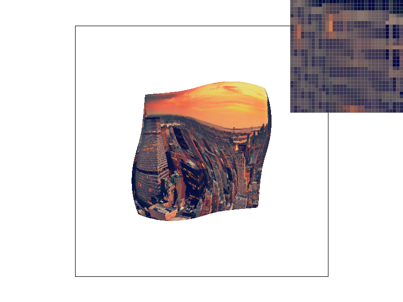
The big Moire pattern on the left most building is gone, compared L_ZERO images.

Attachments

Task 1 Extra Credit Data

Initial implementation

dev322@dev322:~/workfolder/cs184/p1-rasterizer-su20-minos-cs184/build$ ./draw ../svg/basic/test6.svg 
Task1 triangle rasterization duration: 0.00108051
dev322@dev322:~/workfolder/cs184/p1-rasterizer-su20-minos-cs184/build$ ./draw ../svg/basic/test3.svg 
Task1 triangle rasterization duration: 0.0114734

Stride 4 example using rasterize_point on hits rather than rasterize_line which had whole lot of over head, skipping remainders (incorrect view)

dev322@dev322:~/workfolder/cs184/p1-rasterizer-su20-minos-cs184/build$ ./draw ../svg/basic/test6.svg 
Task1 triangle rasterization duration: 0.000796006
dev322@dev322:~/workfolder/cs184/p1-rasterizer-su20-minos-cs184/build$ ./draw ../svg/basic/test3.svg 
Task1 triangle rasterization duration: 0.00884895

Stride 4, same as above with remainders (correct view)

dev322@dev322:~/workfolder/cs184/p1-rasterizer-su20-minos-cs184/build$ ./draw ../svg/basic/test6.svg 
Task1 triangle rasterization duration: 0.00100167
(0.00100167-0.00108051)/0.00108051*100  == 7.2% improvement compared to initial
dev322@dev322:~/workfolder/cs184/p1-rasterizer-su20-minos-cs184/build$ ./draw ../svg/basic/test3.svg 
Task1 triangle rasterization duration: 0.0109772
(0.0109772-0.0114734)/0.0114734*100 == 4.32% improvement compared to initial

with stride 8 (worse performance)

dev322@dev322:~/workfolder/cs184/p1-rasterizer-su20-minos-cs184/build$ ./draw ../svg/basic/test6.svg 
Task1 triangle rasterization duration: 0.00115052
dev322@dev322:~/workfolder/cs184/p1-rasterizer-su20-minos-cs184/build$ ./draw ../svg/basic/test3.svg 
Task1 triangle rasterization duration: 0.0123532

Tags: cs184 cal